The Intelligent Bitcoin Miner, Part II.
April 15, 2021
"Anyone who attempts to generate random numbers by deterministic means is, of course, living in a state of sin."
-- John von Neumann
Overview
In the absence of experimentation, we can fall back on simulation. In tandem with other forms of analysis, simulation can render research on Bitcoin mining tractable despite the industry’s opacity and high capital intensity. It’s expensive to set up an operation without knowing what you’re getting into, but cheap to simulate one.
In Part I of this series, we built a Monte Carlo model to approximate the fair value of mining rigs and the sensitivity of this fair value to different market parameters. We showed that the market price of hashpower often deviates from its theoretical fair value, in part due to the illiquidity of the instrument.
In our last article, we modeled future price trajectory with a Jump-Diffusion process and used a linear function to characterize how global hashpower responds to changes in price. As discussed in several of our articles, though, the dynamic between hashrate and price extends beyond a simple linear relationship. To improve the representativeness of our framework, we have to move beyond characterizing global hashpower as a unit, and instead model it from a bottom-up perspective.
In this article, we characterize miners into several archetypes based on machine type, all-in operating cost, and mining strategy. Each miner archetype has different profit margins and risk considerations. As mining revenue fluctuates, each miner produces a profit or loss that in turn drives their decision to increase or decrease the number of machines operating.
Under this framework, change in network hashrate is not just a function of change in price, but an aggregation of the collective outputs of all miners with distinct economics and risk profiles.
The codebase of the model is entirely open-source, and is available here.
Users can plug in their own assumptions and see how their mining operation would perform under the resulting conditions. In this article, we’ll walk through the model in detail, provide instructions on how to use it, and present some interesting findings from an analysis of five scenarios.
Conway’s Game of Life
Our approach of modeling network hashrate as the sum of individual miners’ outputs is based on a technique called agent-based simulation. Agent-based modeling grew out of John Von Neumann’s early work on cellular automata in the 1950s, and was popularized by John Conway’s Game of Life.
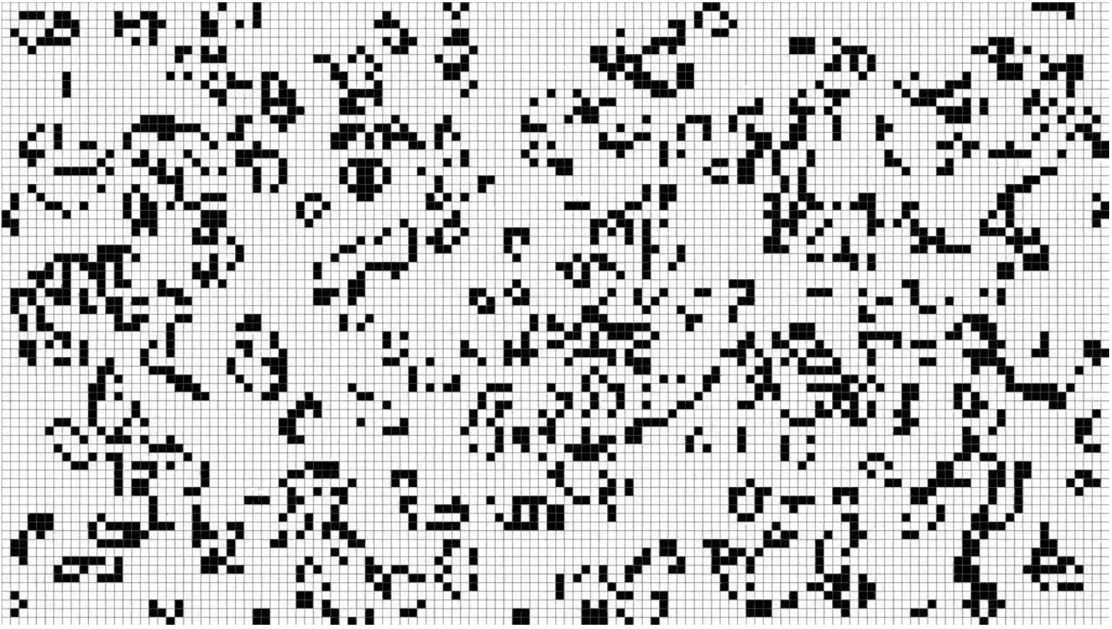
This is a turn-based simulation that takes place on a two-dimensional grid of cells. There are pre-specified, deterministic rules governing the interactions between neighboring cells. With each turn, the status of the cells changes based on the status of that cell's neighbors: cells come to life if they have exactly three live neighbors, stay alive if they have two or three live neighbors, and otherwise die.
The Game of Life is a primitive example of an agent-based model, a type of simulation in which decisions are made by actors sharing a global state. In the Game of Life, the cells are agents, and their decision-making revolves around whether to live or die. The outcome depends entirely on the initial state of the board, and the state of the board can evolve unintuitively.
Agent-based modeling has evolved considerably beyond Conway’s Game of Life. Today, agent-based simulation is widely used in ecology, economics, quantitative finance, and smart contract analysis.
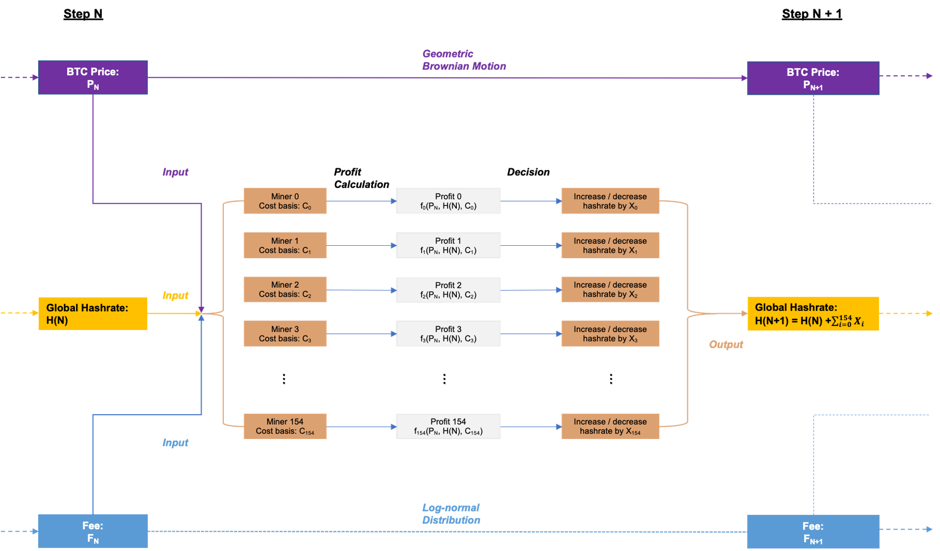
Bitcoin mining profitability is dependent on the price of Bitcoin, the total network hashrate, and to a lesser extent transaction fees (so far). The second component in this profitability calculation, network hashrate, is dependent on other miners’ decisions to run their machines or turn them off. As a result, projections of miner profitability must be iterative, and the problem lends itself well to agent-based modeling.
Assuming Bitcoin price is completely independent of network hashrate, we can model price as a standalone Geometric Brownian Motion. In a similar vein, we model daily fees as independent and log-normally distributed, assuming a constant ten-minute block time.
We regard each day in the time series as a turn; at the beginning of each turn, price, fees, and global hashrate are all fed as inputs to the miner agents’ decision process.
Based on their profit margins, each miner scales their operation up or down by changing the number of machines they run and publishes the hashrate of their operation. The sum of every miner’s hashrate output in turn becomes the new global hashrate:
Miner as Agents
Modeling miners as agents is essentially parameterizing the input variables in mining economics. In The Alchemy of Hashpower, we introduced the concept of the reflexivity of hashpower: every mining operation is heavily affected by both physical conditions and the operator’s subjective perception of the market.
While it is impossible to cover every decision-making factor, we identify Machine Type, Cost Basis, and Strategy as the primary determinants of miner behavior. We formalize these factors as parameters in our miner class.
Machine Type:
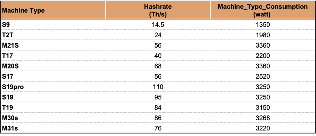
In the real world, a mining operation typically has multiple different types of machines. For simplicity, we have each miner archetype use a single machine type throughout the analysis. In this version of the simulation, we support the following universe of machines:
Cost Basis:
All-in electricity rate
Energy consumption
Each miner is assigned an average all-in electricity rate throughout the simulation. The energy consumption is the miner’s:
Number of Machines * Machine_Type_Consumption.
Each day, the miner incurs operating expense equal to:
Energy Consumption / 1,000 * All-in Electricity Rate * 24.
We also specify an all-in electricity rate distribution, which determines the Number of Machines of the associated miner archetype at initialization.
In this version, we provide the following stratification as default. The user can customize this prior to running the simulation.

(Based on best-effort estimate)
Strategy:
Long BTC
Sell Daily
Each miner is assigned a strategy at initialization. In practice, there is a wide spectrum of strategies miners can use, and they can switch between them whenever their perception of market conditions changes.
For simplicity, we model each miner as following the same strategy throughout the entire simulation. We introduced these two strategies and assessed their performance in different market cycles in The Intelligent Bitcoin Miner, Part I.
Long BTC means that the miner sells only enough to cover operating expenses on a daily basis, and keeps the rest of their revenue in bitcoin.
Sell Daily means that the miner sells everything into USD right away.
A miner’s strategy determines how their USD Position and BTC Position propagate. When calculating the Profit for miners using the Long BTC strategy, unrealized gains need to be taken into account. Unrealized gains are calculated as BTC position * Bitcoin price.
Based on the combination of these three variables, we decompose the universe of miners into 11 machine types, 7 electricity cost strata, and 2 strategies, for a total of 154 archetypes.
At initialization, we provide a default stratification of the machines on the market and price data based on data from Hashrate Index and General Mining Research and a few other sources. The user can customize this prior to the simulation:
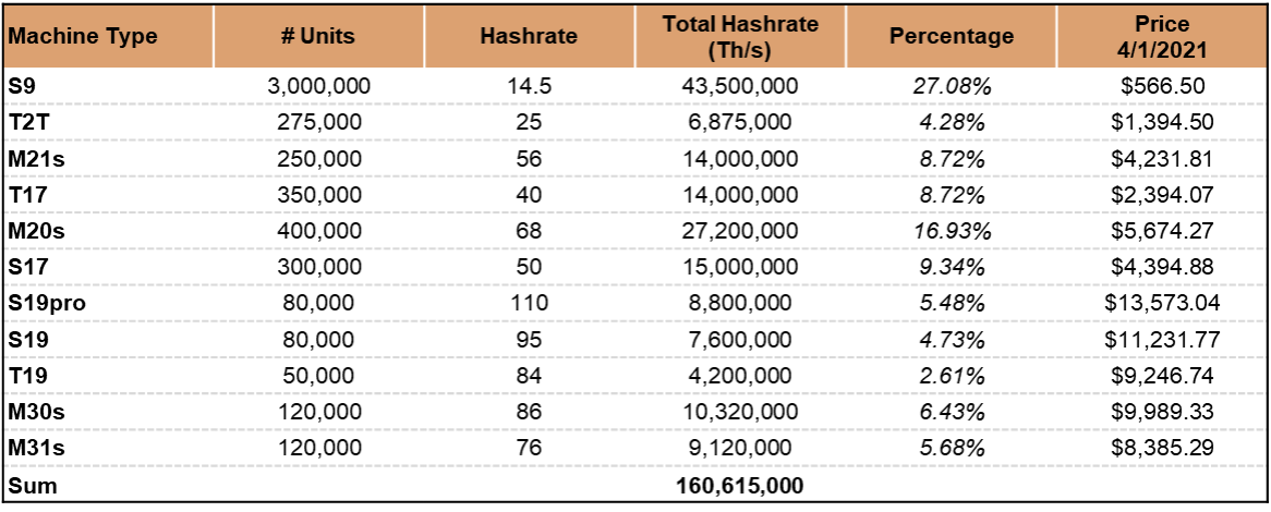
(Price data: Hashrate Index, General Mining Research. Hashrate percentage: best-effort estimate based on various sources)
The Electricity Rate Distribution and the Machine Stratification are inputs in each miner’s Number of Machines. This represents the number of machines that the miner operates. It’s important to note that in practice the two distributions are not statistically independent as assumed in the model—for example, older machines such as S9s are more likely to be operated by miners with access to cheaper electricity.
At the beginning of the simulation, the sum of Number of Machines * Hashrate of all miners is scaled to roughly equal the current network hashrate level, gathered from Coin Metrics.
To track miner performance, we include a simple account balance and historical profit calculator in the miner class.
Account Balance:
USD position
BTC position
Hashpower position
The initial hashpower position is the miner’s Number of Machines * Machine_Type_Hashrate.
Profitability:
Profit_Daily
Profit_Last_30_Day
Profit_All
Profitability determines the miner’s behavior as the market evolves. We will cover the mechanism in the next section. Profit_30_Days and Profit_All are the sums of trailing profits.
Below are all the data entries in a sample miner class. The code for the miner class can be found in the agents.py file.

Miner’s Utility Function
When projected profitability is high, miners may want to purchase more machines, and when expected future profitability is negative, they may turn off some machines to decrease operating expenses. We need to define exactly how miners scale their hashpower up or down.
In reality, there are a number of exogenous factors that drive a miner’s decision to buy more or turn off machines, such as external financing availability and sleep quality. For simplicity, we model the miner’s historical profit as the primary input in the miner’s decision process.
The decision process takes Profit_Last_30_Day as its input, and calculates a result that is used to produce an action. The calculation process is as follows:
If Profit_Last_30_Day is zero or negative, the miner decreases Number of Machines by x until break even. The calculation is simply:
Loss (Profit_Last_30_Day) divided by energy cost per machine.
If Profit_Last_30_Day is positive and exceeds a certain threshold, the miner will increase Number of Machines.
2a) The threshold is: Profit_Last_30_Day > Sum of all (Expenses)
2b) The number of machines to increase is calculated as:
(Profit_Last_30_Day - Sum of all (Expenses)) / Machine Price * Machine Growth Factor
Machine Price is dynamic over the course of the simulation, and is defined as:
Initial Machine Price * (Current Bitcoin Price * Initial Network Hashrate) / (Initial Bitcoin Price * Current Network Hashrate)
Machine prices are adaptive, responding to changes in price and hashrate. Each machine type also has a growth rate that reflects its relative rate of growth. Older generation machines have a smaller rate due to manufacturers’ lack of desire to keep producing them. We also incorporate a reaction delay for adding new machines. It often takes a while for a new order to get manufactured and delivered.
In our model, this means that after an increase of x machines action is triggered, the machines will not immediately get added to the miner’s account.
We set a list of constants as the reaction time for each machine type. The reaction delay is a static approximation, and should be refreshed periodically to reflect changes in supply chain capacity.
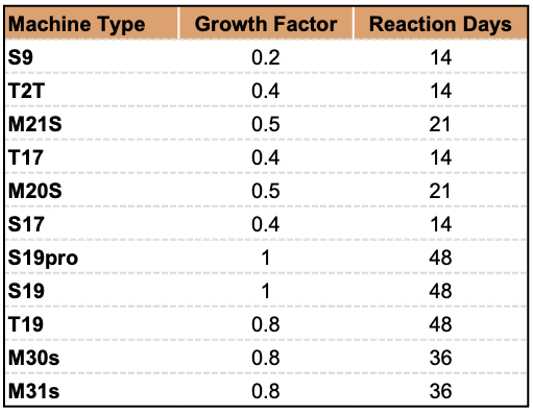
(Based on best-effort estimates)
All told, the trigger function outputs the number of machines the miner is buying or selling.
Users can update the growth factor and reaction times with whatever constants they see fit. The code for the adjustment can be found in Simulator.py.
Setting up the Simulation
As in Part I., we use a stochastic process to project Bitcoin price and daily fee revenue during the lifetime of the simulation. The underlying supports for the Geometric Brownian Motion model for price and the log-normal distribution for fees come from historical price data pulled from Coin Metrics.
Tying everything together, we use the following graph to illustrate how the process works:

Scenario Analysis
To test the model, we simulated different market conditions and analyzed the resulting miner behavior. We assessed the profitability of a user miner who was given $1 million of up-front capital to spend on machines and could not further scale their operation. The simulation was run for 100 days, and the average results from 25 trials were taken.
User profitability was measured at several different electricity costs across our universe of machine types. The highlights are shown below.
The parameters used are by no means definitive, and users are free to re-run the analysis with their own assumptions. The code for the scenario analyses can be found in main.py.
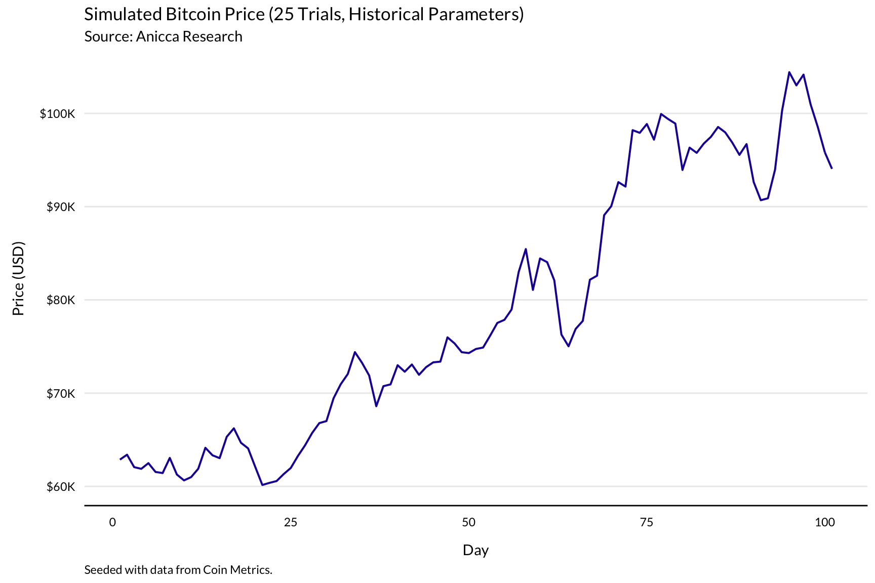
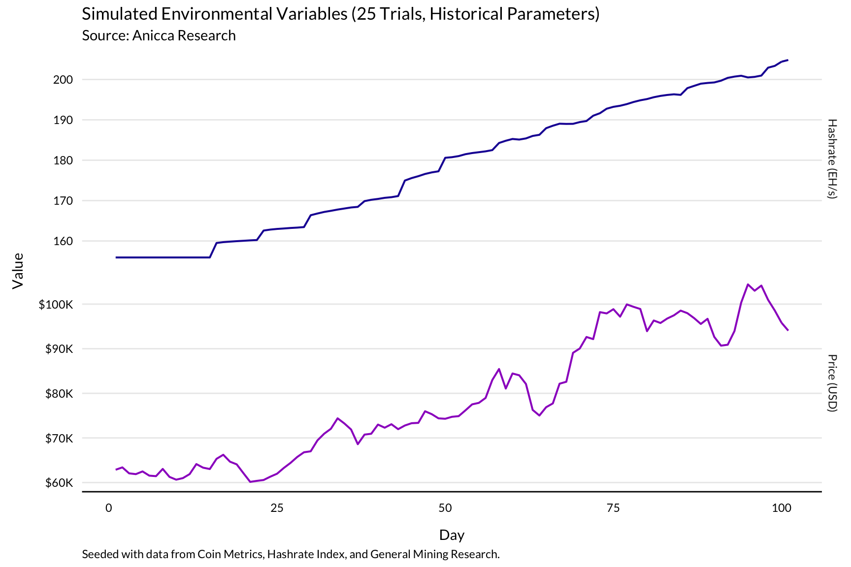
Scenario 1. Bull Market Scenario
Our first test simulates bullish conditions. Given the ongoing bull market at time of writing, we simply fit the Geometric Brownian Motion model to historical data. Under these conditions, price gradually increases to over $100,000, experiencing several corrections along the way.
Network hashrate increases steadily, experiencing some minor lagged corrections in response to downward adjustments in price.

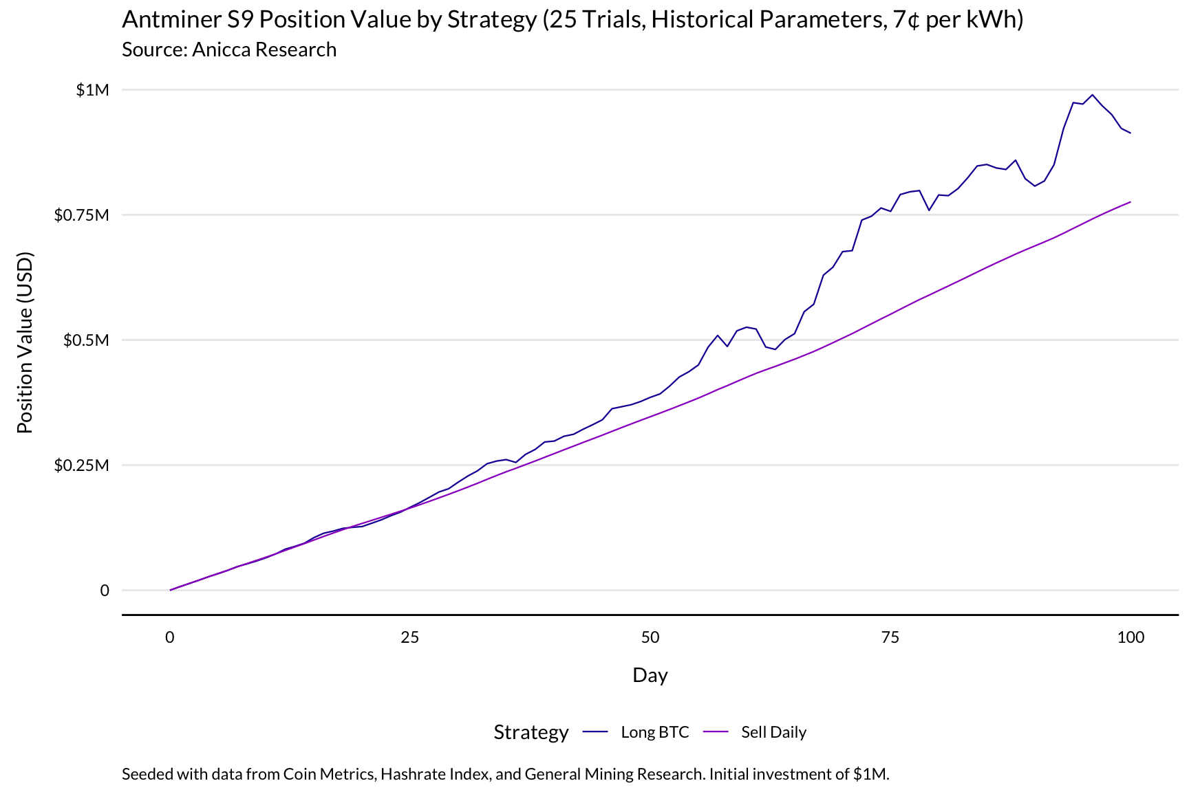
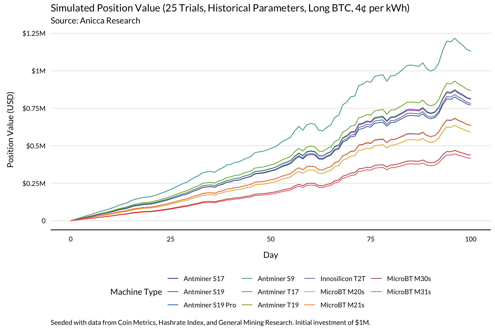
Under these conditions, it’s substantially more profitable to maintain a position in bitcoin than it is to sell daily, even with a high electricity rate. This makes sense given the rapid appreciation in the price of Bitcoin.
At 4¢ per kWh, only miners who use S9s and keep a position in bitcoin break even within the hundred-day simulation period.
Scenario 2. Volatile Market
For our second scenario analysis, we simulate a choppy market by increasing the volatility term in the historically-fit GBM model by 25% and setting the drift to 0. Price initially increases to almost $80,000, before plummeting to slightly over $40,000.

Hashrate begins by increasing rapidly, but starts to plateau in response to the drop in price. Because of the response delay, hashrate continues to increase, albeit more gradually.

Initially, both strategies perform comparably, with bitcoin longs slightly outperforming daily sellers. As price drops, miners with bitcoin exposure are punished for the additional risk they’ve taken on, with the market value of their holdings decreasing.

Scenario 3. Bear Market
The third simulation models a bear market by fitting the GBM to historical data and flipping the sign of the drift term. Price drops dramatically from the current level, nearly hitting $30,000.
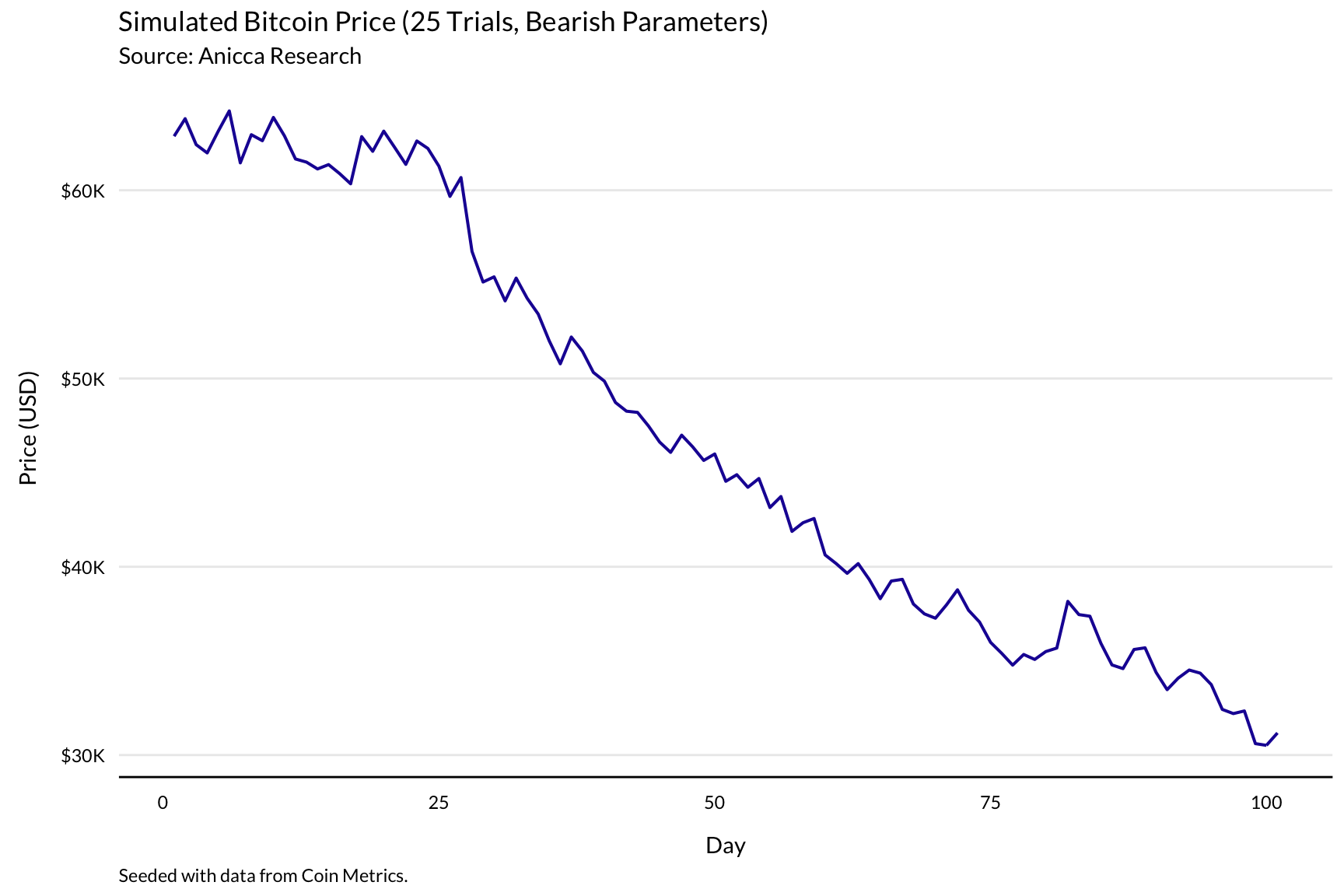
In response to the drop in price, network hashrate enters into a correction after an initial increase. This is the transition from Inventory Flush to the Shakeout phase of the cycle, as introduced in The Alchemy of Hashpower.

In a bear market, everyone suffers. Bitcoin longs are particularly affected: at 4¢ per kWh, the most efficient operations with bitcoin exposure fail to recuperate even half their initial investment within the simulation period.

Daily sellers fare significantly better, but because their earnings are still dependent on the price of Bitcoin, they perform worse than they would have in a bull market.

Scenario 4. In Bull Market, is it better to run old machines or new machines?
The fourth scenario uses the same historical parameters as Scenario 1, with the purpose of comparing the performance of miners running old and new hardware with competitive electricity pricing.
This time, price skyrockets past $140,000, accelerating along the way. Hashrate also increases rapidly.
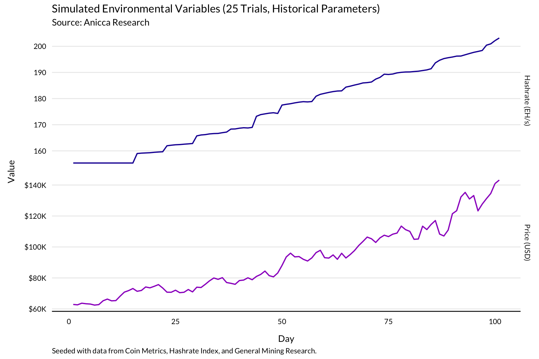
(Scenario 1. vs. Scenario 4.)
Given the intensity of the bull market, even miners who sell daily manage to break even within the hundred-day simulation period, provided they run S9s. S19 miners are significantly less profitable, but still manage to make back most of their initial investment while selling daily.

Miners who are long Bitcoin are incredibly profitable under these conditions. Miners running S9s almost double their investment during the simulation period, and S19 miners also manage to make a substantial profit.

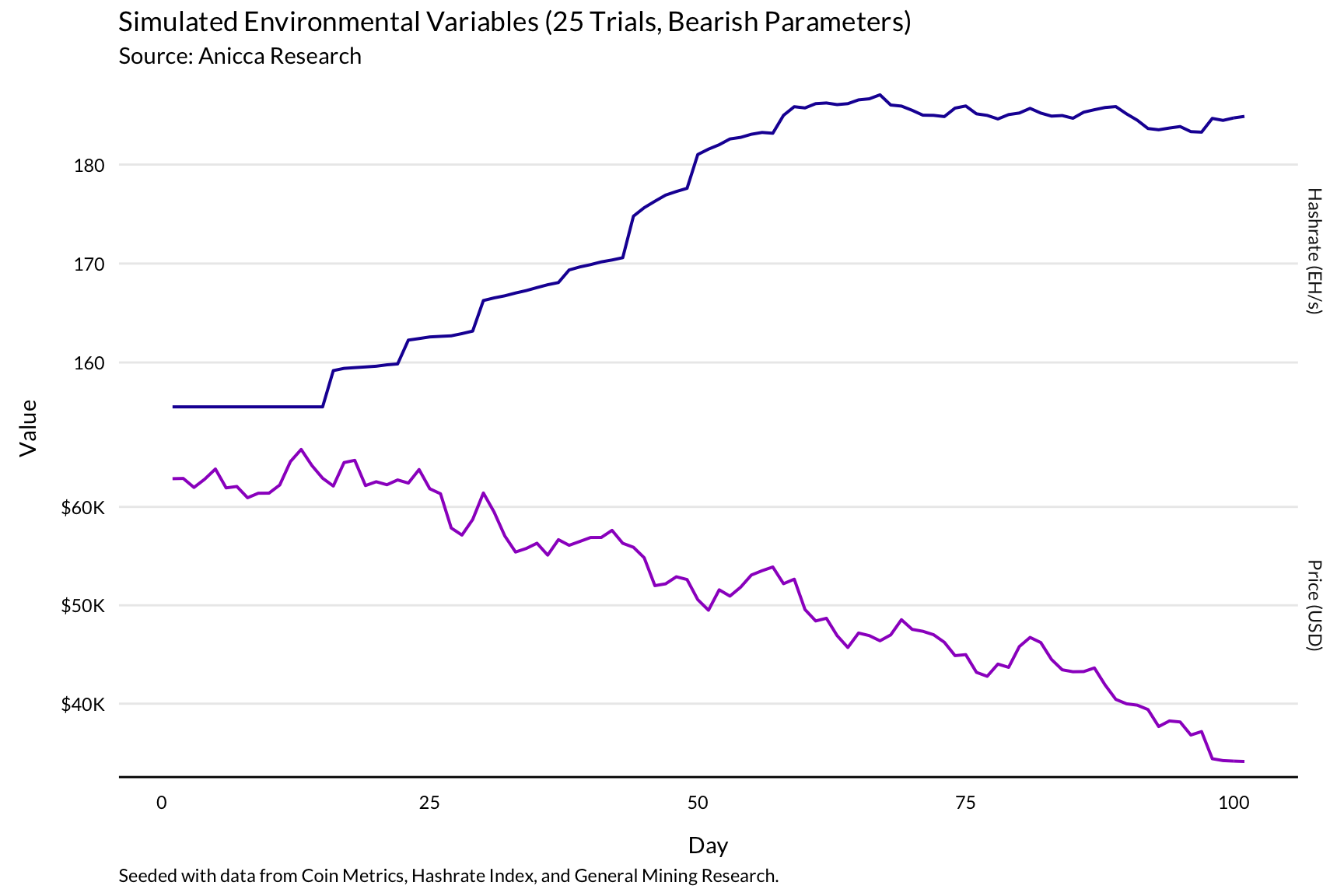
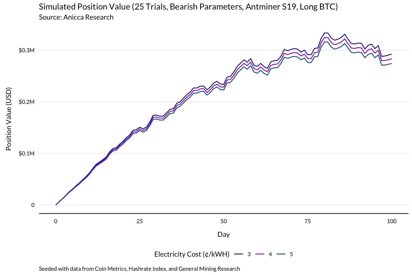
Scenario 5. In a Bear Market, how important is lower opex?
The fifth and final simulation again operates in a bear market, this time with the goal of analyzing the role played by electricity cost in profitability. To do this, we assess the performance of S9 and S19 miners under bearish conditions, with electricity costs of 3, 4, and 5 cents per kWh.
The environment is similar to Scenario 3: price plummets, and hashrate experiences a shallow but prolonged correction.
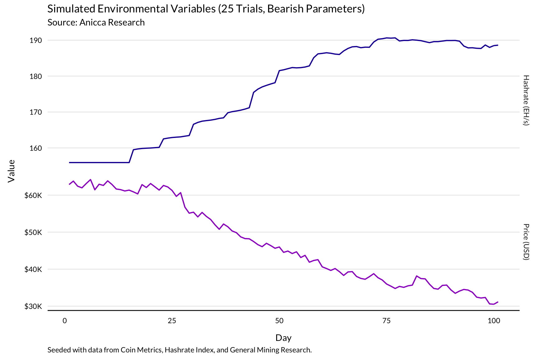
(Scenario 3. vs. Scenario 5.)
For S9 miners, electricity cost makes a substantial difference. While miners at all electricity cost levels perform poorly under these conditions, bitcoin-long miners with 3¢/kWh power manage to make back almost 40% of their initial investment, while their counterparts with 5¢/kWh power make back a little under 32%.

This sensitivity to electricity pricing helps explain why S9 miners tend to operate in frontier regions with cheaper electricity.
For S19 miners, the difference is less pronounced. While miners with lower electricity rates still earn more money than those with higher ones, this variable has a much less significant impact on profitability.
Conclusion
Dimensionality is the statistician’s enemy, and Bitcoin mining is a tough problem to model. Even our model, which makes several simplifying assumptions, managed to grow significantly more complex than we initially intended. Like all Monte Carlo-based tools, its predictive power is fundamentally limited by the biases of the user, which ripple out from the initial seed conditions into any results.
Our model explicitly assumes that the relationship between price and hashrate is unidirectional. Implicitly, it assumes independence between the likely-correlated machine model and electricity cost distributions. All models are wrong, but some are useful.
This model, we think, is useful. It should find its way into the intelligent bitcoin miner’s toolbox.
Acknowledgments
Thanks to Coin Metrics, Hashrate Index, and General Mining Research for data.
Thanks to Guzman Pintos for help accessing and working with rig price data.